# Dr. M. Baron, Statistical Machine Learning class, STAT-427/627

# CROSS-VALIDATION

1. Validation Set Approach

> library(ISLR2)

> attach(Auto); n = length(mpg);

> n

[1] 392

> Z = sample( n, 250 ) # Random subsample of size 250 (does not have to be n/2)

# Works similarly to generating a Bernoulli variable

> reg.fit = lm( mpg ~ weight + horsepower + acceleration, subset=Z ) # Fit using training data

> mpg_predicted = predict( reg.fit, newdata=Auto[-Z , ] )

# Use this model to predict the testing data [-Z]

> plot(mpg[-Z],mpg_predicted) # We can see a nonlinear component

> abline(0,1) # Compare with the line y=x.

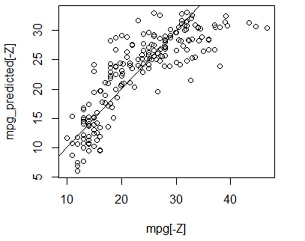
> mean( (mpg[-Z] - mpg_predicted)^2 ) # Estimate the mean-squared error MSE

[1] 18.58128

2. Jackknife (Leave-One-Out Cross-Validation, LOOCV)

“Manually”:

> Yhat = numeric(n)

> for (i in 1:n){

+ reg = lm( mpg ~ weight + horsepower + acceleration, data=Auto[-i,] )

+ Yhat[i] = predict( reg, newdata=Auto[i,] )

+ }

> plot(mpg,Yhat)

> mean((mpg-Yhat)^2)

[1] 18.25595

Using package “boot”:

> install.packages(“boot”)

> library(boot)

> glm.fit = glm(mpg ~ weight + horsepower + acceleration) # Default “family” is Normal, so this GLM model

> cv.error = cv.glm( Auto, glm.fit ) # is the same as LM, standard linear regression.

> names(cv.error) # This cross-validation tool has several outputs

[1] "call" "K" "delta" "seed" # We are interested in “delta”

> error$delta

[1] 18.25595 18.25542

# Delta consists of 2 numbers – estimated prediction error and its version adjusted for the lost sample size due to cross-validation.

# Example – what power of “horsepower” is optimal for this prediction?

> cv.error = rep(0,10) # Initiate a vector of estimated errors

> for (p in 1:10){ # Fit polynomial regression models

+ glm.fit = glm( mpg ~ weight + poly(horsepower,p) + acceleration ) # with power p=1..10

+ cv.error[p] = cv.glm( Auto, glm.fit )$delta[1] } # Save prediction errors

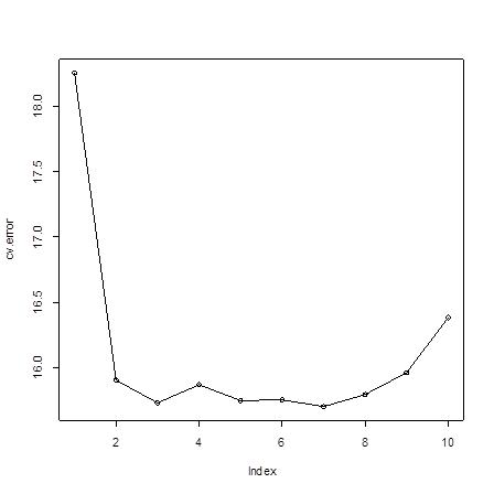
> cv.error # Look at the results

[1] 18.25595 15.90163 15.72995 15.86879 15.74517 15.74989 15.70073 15.79314 15.95933 16.38301

# Although p=7 yields the lowest estimated prediction error, after p=2, the improvement is very little.

> plot(cv.error)

> lines(cv.error)

3. K-Fold Cross-Validation

# We can specify K within cv.glm (Omitted K is K=1 by default, which is LOOCV).

> cv.error = rep(0,10)

> for (p in 1:10){ glm.fit = glm( mpg ~ weight + poly(horsepower,p) + acceleration )

+ cv.error[p] = cv.glm( Auto, glm.fit, K=30 )$delta[1] }

> cv.error

[1] 18.22699 15.87030 15.73565 15.85911 15.80686 15.71585 16.09625 15.67797 15.82097 16.48196

> which.min(cv.error)

[1] 6

4. Cross-validation in classification problems. Loss function.

# Command cv.glm, as we used it above, calculates MSE, the mean squared error, and calls them “delta”.

# In classification problems, MSE can be used to measure the distance between the response variable Y

# and the predicted probability p. For this, Y has to be 0 or 1, and p should be the probability of Y=1.

# However, the correct classification rate and the error classification rate are more standard measures

# of classification accuracy. We can force cv.glm to return these measures by introducing a suitable loss

# function. For example, we’ll be predicting whether a student is depressed or not.

# We define a loss function L(Y,p), a function of true response Y and predicted probability p. The loss = 1 if

# the predicted response is different from the actual response and 0 otherwise. Suppose the threshold is 0.5

> loss = function(Y,p){ return( mean( (Y==1 & p < 0.5) | (Y==0 & p >= 0.5) ) ) }

> loss(1,0.3)

[1] 1

> loss(c(1,1),c(0.3,0.7))

[1] 0.5

# Now we attach the Depression data, skip missing values, fit logistic regression model, and estimate

# the error classification rate by LOOCV.

> Depr = read.csv(url("http://fs2.american.edu/~baron/627/R/depression_data.csv"))

> D = na.omit(Depr)

> attach(D)

> library(boot)

> lreg = glm(Diagnosis ~ Gender + Guardian_status + Cohesion_score, family="binomial")

> cv = cv.glm( D, lreg, loss )

> cv$delta[1]

[1] 0.1615721

# Is Guardian_status significant? Let’s compare the error rates with and without variable “Guardian_status”.

> lreg = glm(Diagnosis ~ Gender + Cohesion_score, family="binomial")

> cv.glm( D, lreg, loss )$delta[1]

[1] 0.1572052

# The error classification rate is lower without the “Guardian_status”.